Datadog Metrics: The Core Concepts for Success

Metrics serve as a cornerstone of observability, providing invaluable insights into the performance and health of systems, applications, and infrastructure. One of their greatest advantages lies in their ability to be effortlessly stored over extended periods. This capacity for long-term retention enables organizations to analyze historical trends, identify patterns, and make informed decisions based on past data.

Yet, the true power of metrics transcends mere storage capabilities. Beyond their technical utility, with custom metrics users can bridge the gap between technical and business realms, facilitating the convergence of technical information with crucial business insights. By combining technical metrics with business-oriented data points, companies can gain a holistic understanding of their operations, uncovering opportunities for optimization, innovation, and strategic growth.

In this blog post, we delve deeper into the core technical concepts to master around custom metrics to improve the quality of your dashboards and monitors and optimize usage.

What is cardinality? How is it proportional to cost?

Cardinality means the number of elements in a set or other grouping, as a property of that grouping. In the case of a metric, this is related to the number of contexts that are received.

In the case of Datadog, we measure cardinality with

“A custom metric is uniquely identified by a combination of a metric name and tag values (including the host tag)” — doc

In practice

In other words, for each combination of tags (or context), Datadog will store a timeseries. For instance, if 5 hosts are each reporting the disk space free, Datadog will store 5 timeseries for each of the 5 hosts:

• host:apple
• host:pear
• host:banana
• host:peach
• host:blueberry

Now the interesting part comes when you add tags. Let’s assume that each host belongs to one unique environment. In that case, even though we add information, we still have 5 unique contexts:

• env:prod, host:apple
• env:prod, host:pear
• env:prod, host:banana
• env:preprod, host:peach
• env:staging, host:blueberry

The number of potential combinations is larger but the number of reporting combinations of tags is still limited to 5.

Now, let’s assume the hosts in env:prod have 2 disks and the other hosts have only one. We would like to then get the disk space free for each disk. In that case, this adds some new combinations:

• env:prod, host:apple, disk:a
• env:prod, host:apple, disk:b
• env:prod, host:pear, disk:a
• env:prod, host:pear, disk:d
• env:prod, host:banana, disk:b
• env:prod, host:banana, disk:c
• env:preprod, host:peach, disk:a
• env:staging, host:blueberry, disk:c

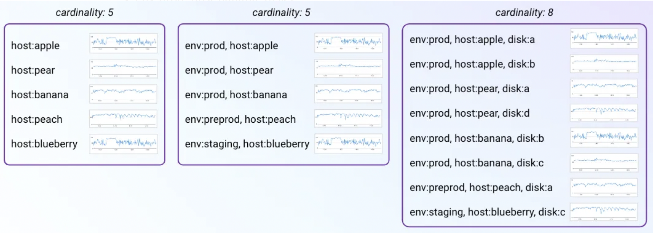
In conclusion, for this section, the combination of tags is what really matters because for each combination a timeseries will have to be stored. Now, what we’ve seen with the examples above, adding a tag does not always add cardinality. So feel free to use such knowledge to your advantage.

Types with their aggregation and interpolation

As metrics become more and more used, the knowledge of metric types and their default behavior is critical to build accurate dashboards.

To get started, it is important to note that 2 aggregations can happen:

• time aggregation: the ability to consolidate multiple data points over a time period into a single point.
• space aggregation: the ability to consolidate multiple data points from multiple contexts (i.e. combination of tags) into a single point.

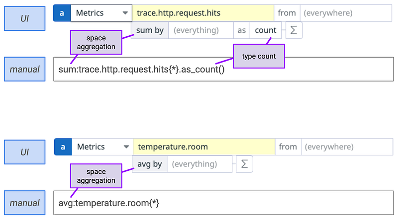
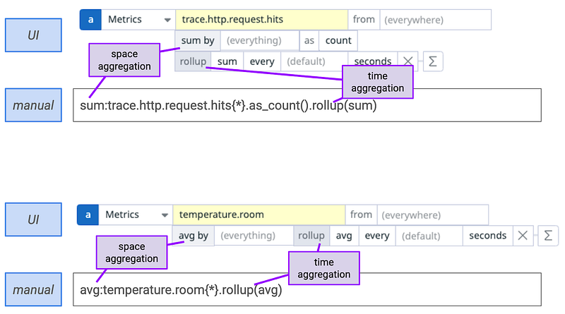
The default aggregation will differ depending on the metric type. Let’s focus here on the most common types: count and gauge with an example. The count metric will be represented by the number of hits on my service. The gauge metric will be represented by the room temperature.

In practice

Let’s start with the count metric that will be named: trace.http.request.hits. Some interesting stats to collect are:

• space aggregation: the hits for all my endpoints. In this case, the default space aggregation will be a sum.
• time aggregation: the hits on endpoint:/home for the whole day. In this case, the default time aggregation will be a sum.

Now, let’s look at the gauge metric that will be named: temperature.room. Some interesting stats to collect are:

• space aggregation: the temperature for all my rooms. In this case, the default space aggregation will be an average.
• time aggregation: the temperature of room:living_room for the whole. In this case, the default space aggregation will be an average.

It is now clear to see that for the metrics of type count, the preferred aggregation is sum whereas for metrics of type gauge the preferred aggregation is average. If we now look in Datadog, the time aggregation is by default hidden but can be overridden with a rollup function.

Now that the concept of aggregation is understood, the other important underlying behavior behind metrics is the concept of interpolation. For that part, the Datadog doc explains such concept in 2 brief sections.

From histograms to distributions

This section is quite focused on Datadog capabilities and how the distribution metric introduced a few years ago is greatly improving the experience of manipulating the data for high volume applications.

Let’s go back to the basics, when an application reaches a certain scale, gauge and count metrics no longer answer all meaningful questions at an optimized cost. For instance, storing each individual latency of a service receiving 1,000 requests/sec is not scalable. In addition, no one will have time to look at all those requests individually. That’s why, the concept of histograms has been introduced. In Datadog, the definition is: The HISTOGRAM metric submission type represents the statistical distribution of a set of values calculated Agent-side in one time interval. — doc. On OpenMetrics, users also have to understand the concept of buckets.

# HELP http_request_duration_seconds Histogram of latencies for HTTP requests. 
# TYPE http_request_duration_seconds histogram 
http_request_duration_seconds_bucket{handler="/",le="0.1"} 25547 
http_request_duration_seconds_bucket{handler="/",le="0.2"} 26688 
http_request_duration_seconds_bucket{handler="/",le="0.4"} 27760 
http_request_duration_seconds_bucket{handler="/",le="1"} 28641 
http_request_duration_seconds_bucket{handler="/",le="3"} 28782 
http_request_duration_seconds_bucket{handler="/",le="8"} 28844 
http_request_duration_seconds_bucket{handler="/",le="20"} 28855 
http_request_duration_seconds_bucket{handler="/",le="60"} 28860 
http_request_duration_seconds_bucket{handler="/",le="120"} 28860 
http_request_duration_seconds_bucket{handler="/",le="+Inf"} 28860 
http_request_duration_seconds_sum{handler="/"} 1863.80491025699 
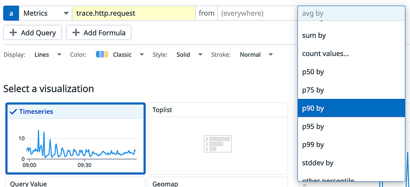
http_request_duration_seconds_count{handler="/"} 28860

Understanding such output needs training and handling such data to know when the p90 is above 3s is quite complex. Datadog then introduced the concept of distribution metrics. This heavily simplifies the manipulation and reading of the data. To get information about the p90, p95 or any custom percentile, only the space aggregation has to be changed without any need for some mathematical formulas.

The math and concepts applied to offer such smooth UX has been well detailed in this blog post.

The benefit of distribution extends to the ability of controlling tags within Datadog UI and thus controlling what is stored (and consequently its cost). Do not hesitate to abuse such features for distribution metrics.

Metrics without Limits™

Having the finest level of detail for all tags and aggregations across every metric may not always be beneficial. That’s why Datadog introduced Metrics without Limits™ (MwL). Metrics without Limits™ gives control over custom metric volumes by separating custom metric ingestion from indexing. This allows teams to only pay for valuable custom metric tags.

However, it’s advisable not to send such metrics or tags in the first place. But this can be challenging when responsibilities are divided, when the application is in production and can’t be easily restarted, or when there’s an urgent need to reduce data volumes.

Since most decisions to use MwL are driven by cost considerations, although metric ingestion becomes billable with MwL, the cost of ingestion is typically much lower compared to the indexing cost. Therefore, savings at the indexing level usually outweigh any increase in ingestion cost.

In practice

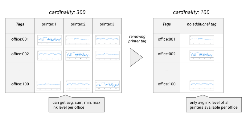
Let’s illustrate how MwL works with an example. Consider monitoring ink levels in printers across multiple offices. The metric name is printer.level, and we have 100 offices (tag: office) each with 3 printers (tag: printer).

Initially, without any tag manipulation, we have 300 custom metrics reporting (100 offices * 3 printers). Suppose we’re only interested in the average ink level per office, so we can drop the printer tag. Using Metrics without Limits, we reduce the number of contexts to 100, one for each office. Datadog will store the average ink level of all printers per office. The number of custom metrics now drops to 100.

Now, let’s say the office management wants to know if any printer’s ink level drops below 5ml. With MwL, we can add a new space aggregation to track the minimum ink level across offices. This results in 100 contexts for average ink levels and another 100 for minimum ink levels per office, totaling 200 contexts.

Overall, MwL is a powerful tool, but it requires understanding its implications in terms of stored information. If, for instance, we also want to track the total ink level across all printers in an office and the maximum ink level per office, the cardinality increases to 400, compared to the original 300 which would remove any benefits originally gained. MwL is beneficial in 90% of cases aiming to reduce costs, but its underlying concepts must be grasped for maximum efficiency and avoid costly mistakes.

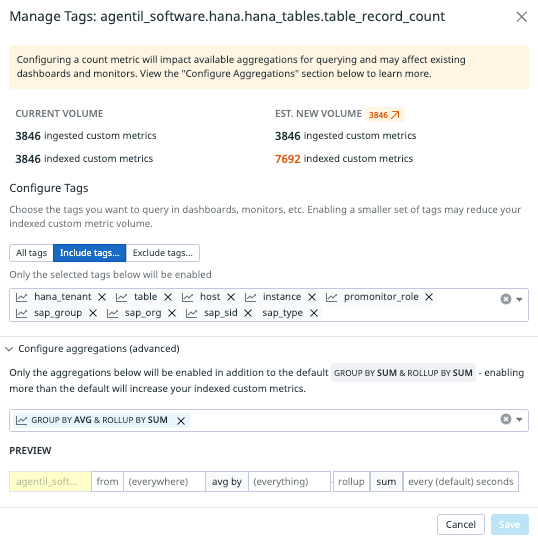
If you are unsure, the UI will provide instant feedback on the expected cardinality based on recent data. In the example below, we can clearly see that the number of indexed metrics will actually increase.

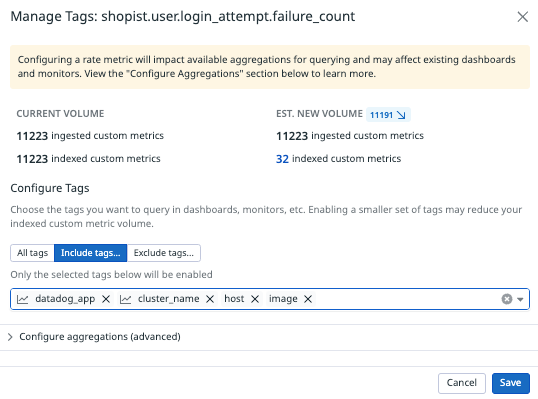
Whereas in this other example, the indexed custom metric count is heavily reduced. Note that Datadog will automatically select tags based on their recent utilization. If they have not been used recently, it will not pre-select them.

Doc and Blog post

When and how to leverage MwL?

As described above, Datadog offers a great set of tools to reduce the cardinality of individual metrics. At scale, the method advised to tackle custom metric reduction is:

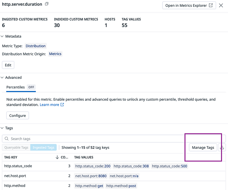
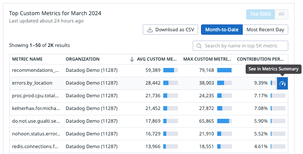
1. Go to the plan and usage page and go to the custom metric tab

2. Open the top custom metrics in the metric summary page

3. For each of those opened metrics, click on manage tags to identify if the indexed metric count would actually drop.

4. Then make a decision based on the knowledge you just acquired.

In conclusion, metrics stand as indispensable tools in the realm of observability, offering organizations a window into the inner workings of their systems and infrastructure. Their inherent capability for long-term storage ensures that valuable data is preserved, allowing for retrospective analysis and continuous improvement over time.

To ensure an optimal use of such metrics, mastering the underlying behaviors of different metric types is essential as well as mastering the ability to manipulate tags from the UI.